The Atlas of Living Australia spatial portal now includes additional tools for exploring the environmental parameters which influence the distribution of each species. These tools often suggest interesting questions about the biology of the species. This post is to show the use of these tools, illustrated with the example of Eucalyptus camaldulensis Dehnh. (River Red Gum).
Here is the spatial portal map for all records of Eucalyptus camaldulensis:
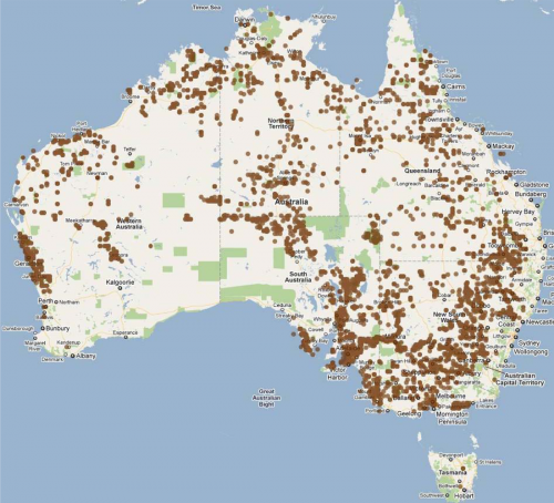
Each dot on this map represents a location where a specimen or observation has been identified as belonging to this species. Clearly this is not a full view of the range of the species in Australia, and doubtless there are some records here which may have been misidentified. Nevertheless this is a rich sample of the locations where the species occurs – and the environment at each of these locations is a sample of the environments which can support this species. The ALA spatial portal includes over 300 different geospatial layers for use in modelling and analysis. We can sample these layers to get values for annual mean temperature, annual rainfall and many other factors at each of the locations where Eucalyptus camaldulensis has been recorded.
The download tools included within the spatial portal make it easy to get a spreadsheet of records for any species with every record annotated with these environmental parameters. A new scatter plot tool makes it possible to visualise and explore this information in new ways. Right now this tool can be found under the Analysis tab and the Scatter plot sub-tab, although this is likely to change as the portal develops.
The scatter plot tool requires three choices to be made – the species to be analysed and a selection of two environmental layers to provide values for the scatterplot. Here is the scatter plot for Eucalyptus camaldulensis localities based on “Precipitation—annual seasonality” and “Temperature—annual mean (Bio01)”:
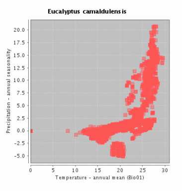
The graph shows how the recorded locations for this species are distributed through an abstract plane defined by rainfall seasonality and mean temperature. The records at (0, 0.0) are from locations which fall outside the area covered by the environmental layers – the supplied coordinates for these localities fall offshore (incorrect or imprecise coordinated).
Clearly there is a significant disjunct cluster at the bottom of the scatter plot. This gap around this cluster represents a set of environments (defined simply by the selected properties) for which we have no records of Eucalyptus camaldulensis – even though we have records of the species occupying environments on either side of this set of environments. (Another way to consider this would be to focus on locations with the same value for annual mean temperature, for example 20C, and consider the spread of values for rainfall seasonality at these locations – the distribution would be bimodal, with complete separation between two clusters.) This immediately poses the question of why the species is not found at locations with intermediate environments.
One possible answer would be that our sample of locations for the species is too incomplete to be fully representative. Given the number of records for this species from right across Australia, this is possible but seems unlikely.
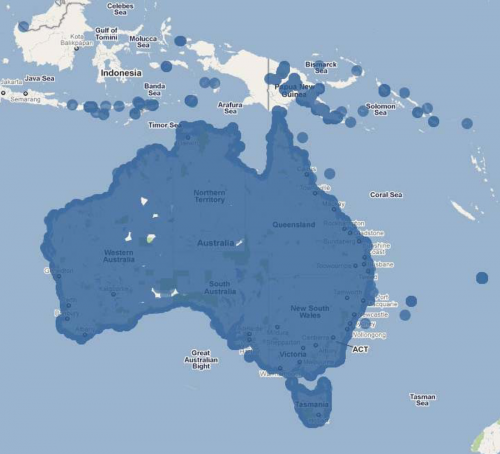
Another possible answer could be that what we are seeing is simply a result of Australian geography. It could be that the Australian landmass does not include any areas with intermediate environments of this kind. This can quickly be disproven. Here is the occurrence map for all species of parrot (Psittacidae) in Australia, along with the equivalent scatter plot:
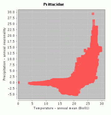
Some species of parrot can be found just about everywhere in Australia and the scatter plot therefore shows us the whole spread of environments which can be found in Australia. There is no discontinuity in this scatter plot, which suggests that there is indeed something significant about the discontinuity in Eucalyptus camaldulensis distribution. A possible enhancement to the scatter plots would be to colour the background to indicate which environmental combinations are possible within Australia.
It is possible to use the scatter plot tool to select records matching a portion of the environment. Simply left-click on a position in the graph and drag a rectangle around the section of interest. This will cause the corresponding locations on the map to be highlighted in red. Doing this for the cluster at the bottom of the E. camaldulensis scatter plot highlights a number of locations in the south-west of Western Australia:
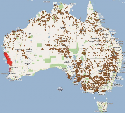
This tool cannot take us much further, but it is possible to hypothesise what is happening. The locations indicated here fall within the hybridisation zone between Eucalyptus camaldulensis and its close relative Eucalyptus rudis Endl. (Flooded Gum). The underlying records come from specimens in Australia’s Virtual Herbarium and have been formally identified as Eucalyptus camaldulensis, so the issue is not that the plants have been misidentified. Perhaps hybridisation has introduced genes into the population which support growth in environments to which Eucalyptus camaldulensis is in general unsuited. Another alternative might simply be that Eucalyptus camaldulensis is elsewhere excluded from this kind of environment because of interspecific competition or some other factors not identified here. In any case, simple exploration of species occurrence data in multiple dimensions can lead us to ask new and interesting questions.
Tools like this have many possible uses:
- It becomes possible to make quick visual comparisons between the environmental niches for different species – we are exploring the possibility of adding a “dashboard” of several standardised environmental scatter plots (e.g. rainfall vs. temperature, solar radiation vs. rainfall, solar radiation vs. temperature) to each species overview.
- Understanding the environmental “niche” for any species allows us to identify areas where the species might successfully survive. This has application in conservation (understanding where it may be possible to maintain safe populations of threatened species), in biosecurity (understanding where invasive species may be able to survive) and in agriculture (understanding where varieties of crop plants may grow successfully).
- Where a species tolerates a wide range of environments, there is likely to be underlying genetic variation which supports this tolerance. As species become pressured under climate change, these tools would allow researchers to identify populations within a species which might be best adapted to survive in future environments.