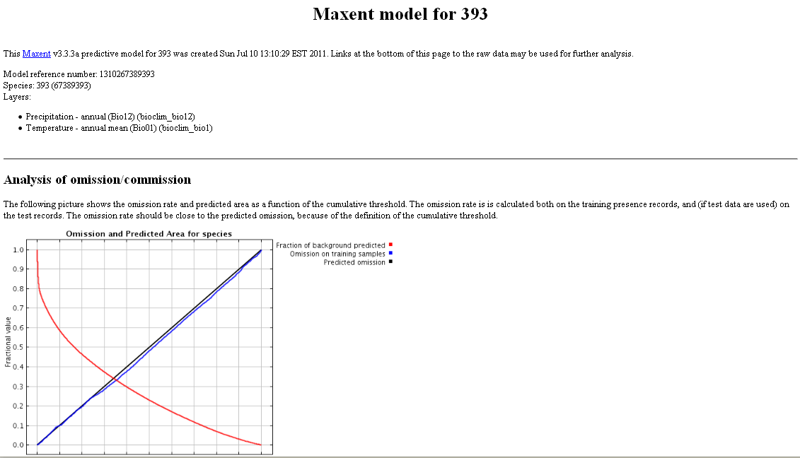
The Predict option under the Tools Menu helps you to identify where a species could occur – not just where it has been observed!
The method used is called “MaxEnt” for Maximum Entropy and was developed by Stephen Phillips.
See (Maxent software for species habitat modeling).
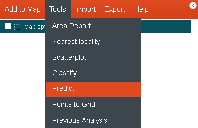
To start a Prediction, select from the Menu Option, “Tools”, then “Predict”.
MaxEnt looks at where species occur in terms of location and environment, and also where the species does not seem to occur. A model is built using the available species and environmental data and the result is essentially, a probability surface showing where the model suggests the species could occur.
You need considerable expertise in modelling, to understand the environmental variables and areas to factor into the prediction tool. Only then can you extrapolate any meaning into the results of the predictions.
Important: The area used for the prediction will be the defined active area. If you have not specifically defined an active area, then the current map extent in the mapping window forms the active area. This is extremely important in prediction as you will not want to extrapolate too far beyond the environmental conditions where the species occurs. It is strongly recommended that you circumscribe the active area to fit the occurrence locations as well as cover the area of interest (which may extend beyond the mapped occurrences). This is always the trade-off!
Run the Prediction Wizard
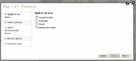
(Please refer to Add Area for additional information).
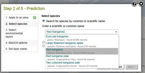
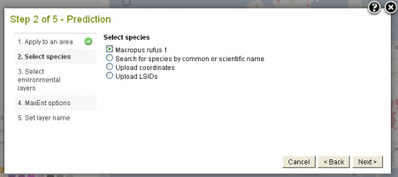
The auto-complete section mechanism is the same as on the Add to Map ->Species. Type the first three letters using either a scientific or common name and a list of suggestions is produced. Select a species (or higher taxonomic class) by clicking on it. The number of occurrences is given alongside the species (or higher taxonomic class).
Selected species will be mapped, if not mapped previously. See Add to Map ->Species.
The last mapped species (or genus, family or order) is included as a species selection choice in Step 2 of 5 of the wizard. (See image below).
Species can also be uploaded using two other methods:
- Upload points. More info »
- Upload LSIDs. More info »
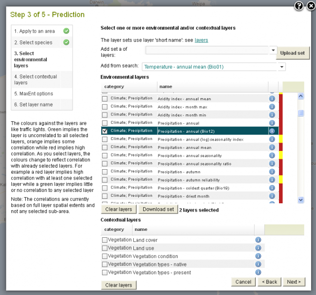
Prediction is mainly based upon environmental layers, but after some research a new version of MaxEnt is able to accept a subset of the contextual layers as predictors. The contextual layers available for prediction are:
- Land cover
- Land use
- Vegetation – condition
- Vegetation types – native
- Vegetation types – present
The selection of appropriate layers is extremely important if an effective model is to be built. The Spatial Portal has around 300 layers covering an extremely wide range of environmental and contextual variables that experts believe could have some control on the distribution of organisms. Many of these variables / layers are highly correlated. If highly correlated layers are used, the model will be weighted accordingly by those variables, regardless of how ‘intelligent’ the method. It always pays to know your organisms well! Know what environmental and contextual factors can influence or control their distribution.
NOTE: The relationships between the layers for the colour coding has been calculated at the national extents. Layers may therefore be more or less related at different scales.
Every layer added to the model may improve it, or over-fit it. To assist, the Spatial Portal has built a form of correlation between all its environmental layers. When a layer is added to the model, the Portal examines the relationship between it and all other environmental layers. It then colour codes the remaining layers in ‘traffic light’ colours. Green against a layer suggests that there appears to be (not necessarily ‘is’) little correlation between that layer and the selected layer. Orange is intermediate while red suggests that there is a fairly high correlation. Remember that while there may be a high correlation, a layer may still have a subtle different factor that may be important. When a new layer is added, the colours are re-calculated on the basis of the closest relationship to any existing layer added to the model.
Other traps for the unwary include using occurrences that have a wide range of observation dates. In this case, the model may be poor because of migration, changed environments or even evolution. A key issue is that the species should be in equilibrium with the environmental variables. The worst case may occur with an invasive species where it’s spread may be rapid and where it is far from reaching ‘environmental equilibrium’.
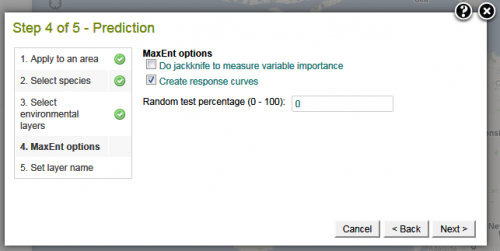
- Jacknife in MaxEnt – selecting this option examines the significance of the environmental variables – one at a time. Jacknife tests identify environmental variables with highest gain when used in isolation. High-gain variables have the most useful information when used by themselves. The environmental variable that decreases the gain the most when it is omitted has the most information, that is not obviously present in the other variables.
- Each model is assigned a unique identifier that allows it to be displayed in subsequent sessions e.g. Model reference number: 1310016793060. This value is given in the metadata of the layer. The Restore Prior Analysis tool uses this identifier to restore a model created earlier. It can be from a totally different session, browser or even PC.
- Create response curves. This option creates a graph for each layer value (x-axis) against probability (y-axis). These curves are useful for evaluating how well the selected layers have captured the species environment.
- Random test percentage. This option allows the user to define the percentage of the occurrences for testing against the output model.
- See in the Referenced Links a tutorial on running MaxEnt.
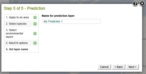
Click on the ‘Next’ button to run MaxEnt.
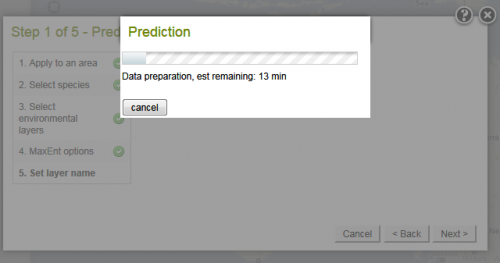
The map window becomes grayed-out and a Prediction data preparation and running time dialogue popup appears on the screen, to indicate how long it should take before the MaxEnt output is displayed.
Note: Building a MaxEnt model can take some time. The time is dependent on a combination of factors: the number of occurrences, the size of the geographic extent of the model, and the number of environmental layers selected.
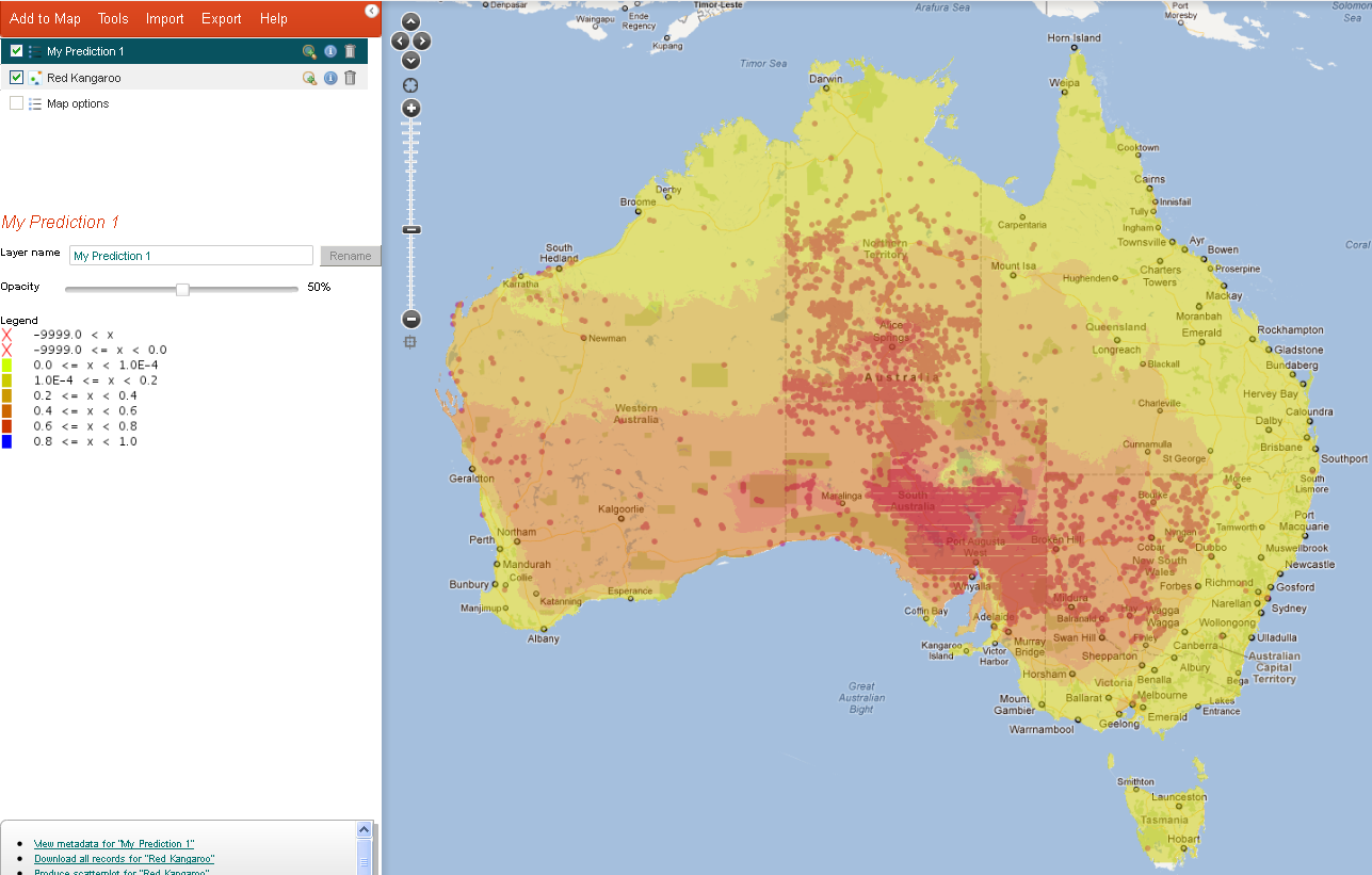
The map is not included in MaxEnt results zip file, as might be expected. The reason for this omission is to hide the location of potentially sensitive species. The Spatial Portal does however display the prediction map – and as with all mapped objects, this layer is added to the list of active layers.
Metadata
When the layer metadata icon ![]() icon is clicked in the layers list the metadata popup is displayed for the Prediction layer. The metadata can be displayed in a separate window.
icon is clicked in the layers list the metadata popup is displayed for the Prediction layer. The metadata can be displayed in a separate window.
The metadata and the results from the prediction. Click to see the Model Reference Number.
The Model Reference number used to restore prior analysis is shown at the top of the metadata.
The metadata contains the methods and modelling used to create the prediction. Response graphs show the impact each of the chosen environmental layers had on the prediction. An image of the prediction probability map layer is also included.
A Case Study
A case study on using the MaxEnt Prediction tool to predict the distribution of the Greater Glider, was prepared by Dr Jane Elith, of The University of Melbourne.
Read the Case Study »
References
- Elith, J., Phillips, S.J., Hastie, T., Dudik, M., Chee, Y.E. and Yates, C.J. (2011). A statistical explanation of MaxEnt for Ecologists. Diversity and Distributions, 17, 43-57.
- Phillips, S.J., Dudík, M., A and Schapire, R.E., Maximum entropy approach to species distribution modeling PDF (185 KB)
- Phillips, S.J., Anderson, R.P. and Schapire, R.E., 2006. Maximum entropy modeling of species geographic distributions. Ecological Modelling, vol. 190, pp. 231-259. PDF (902 KB).
- Phillips, S.J., A Brief Tutorial on Maxent. Word (4.3 MB).
Demonstration Youtube Video
By Lee Belbin, Geospatial Team Leader
